Attractor Switching for Nonlinear Dynamical Systems Using Deep Reinforcement Learning

• NOTE: This page is a brief introduction of a published work. The detailed information can be found on arXiv and Journal of Vibration and Control.

Abstract

• This work describes an approach for attractor switching (or multi-stability control) in nonlinear dynamical systems.
• Attractor switching is realized using two different deep reinforcement learning methods: the cross-entropy method (CEM) and the deep deterministic policy gradient (DDPG) method.
• Experiments were performed on a Duffing oscillator, which is a classic nonlinear dynamical system with multiple attractors.
• DDPG exhibits faster learning, lower performance variance, and smoother control than CEM.

Background and Motivation

Coexisting solutions (or attractors) are a hallmark of nonlinear systems and appear in highly disparate scientific applications. For these systems with multiple attractors, there often exists a preferable solution and one or more less preferable, or potentially catastrophic, solutions.

Various applications with coexisting attractors motivates the development of control methods to switch between attractors. Generally, switching between attractors has to deal with highly-nonlinear behaviors, physical control constraints and optimization of control effort (e.g. energy, time, money, human labor, etc). Reinforcement Learning (RL), as an approach to nonlinear optimal control, is therefore selected to realize attractor switching in nonlinear dynamical systems.

Reinforcement Learning Framework

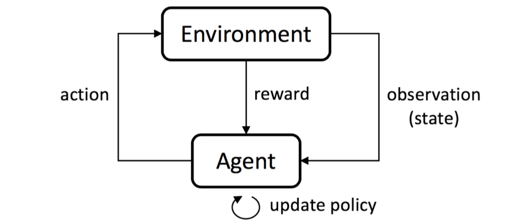
In the reinforcement learning (RL) framework shown in Fig. 1, an agent gains experience by making observations, taking actions and receiving rewards from an environment, and then learns a policy from past experience to achieve goals (usually maximized cumulative reward).

Figure 1. The typical framework of Reinforcement Learning. An agent has two tasks in each iteration: (1) taking an action based on the observation from environment and the current policy; (2) updating the current policy based on the immediate reward from environment and the estimated future rewards.

This work implements RL algorithms to realize attractor selection (control of multi-stability) for nonlinear dynamical systems with constrained actuation. As a representative system possessing multiple attractors, the Duffing oscillator was chosen to demonstrate implementation details.

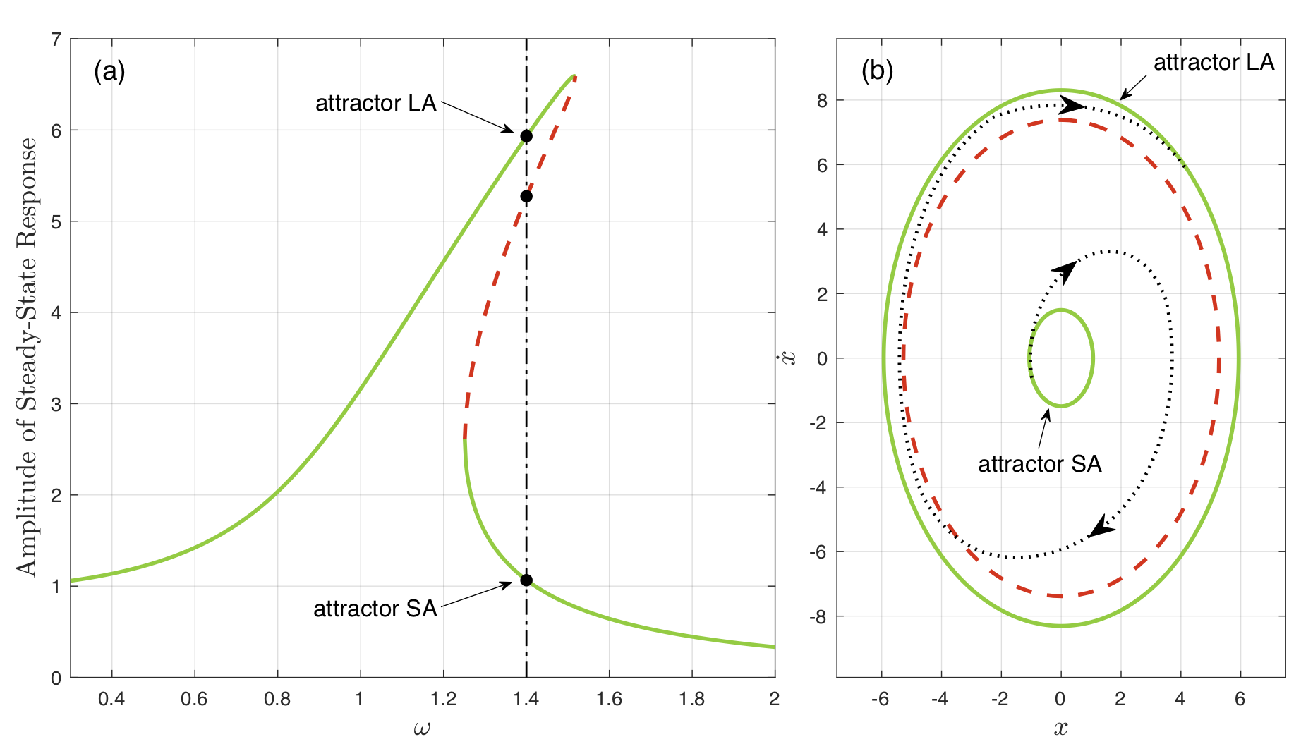
A harmonically forced Duffing oscillator can be described by the differential equation \(\ddot{x} + \delta \dot{x} + \alpha x + \beta x^3 = \Gamma \cos{\omega t}\). Fig. 2 shows an example of coexisting stead-state oscillations. With a long-run time evolution, the oscillation of the unstable solution cannot be maintained due to inevitable small perturbations. The system will always eventually settle into one of the stable steady-state responses of the system, which are therefore considered attractors. Our objective is to apply control to the Duffing oscillator to make it switch between the two attractors as the dotted line in Fig. 2(b).

Figure 2. Coexisting attractors for a hardening Duffing oscillator. (a) Frequency responses. (b) Phase portrait of coexisting solutions when frequency = 1.4. Within a specific frequency range, periodic solutions coexist in (a), including two stable solutions (green solid lines) and an unstable solution (red dashed line) in-between. The stable solutions correspond to an attractor with small amplitude (SA) and one with large amplitude (LA). The dotted line in (b) is a trajectory of switching attractor SA-to-LA using the control method introduced in this work.

To provide actuation for attractor selection, an additional term \(a(s)\), is introduced into the governing equation:

\[\ddot{x} + \delta \dot{x} + \alpha x + \beta x^3 = \Gamma\cos{ \left( \omega t + \phi_0 \right) } + a(s),\]

where, in terms of RL, this equation itself is the environment, \(a(s)\) is the action which depends on the state \(s\). For example, if the Duffing oscillator is a mass–spring–damper system, \(a(s)\) represents a force. The last (also the most important) element in RL is the reward function \(r(s_t, a_t)\), which can be written as:

\[r(s_t, a_t) = -|a_t| \Delta t + \begin{cases} r_\text{end}, & \text{if $s_{t+1}$ reaches the target attractor,}\\ 0, & \text{otherwise.} \end{cases}\]

The action cost is defined as the impulse given by the actuation, \(\lvert a_t \rvert \Delta t\), where \(\Delta t\) is the time step size for control. The environment estimates whether the target attractor will be reached by evaluating the next state \(s_{t+1}\). A constant reward of \(r_\text{end}\) is given only if the target attractor will be reached.

Results

The control policy for attractor switching was learned by using two RL algorithms: 1) cross entropy method (CEM) and 2) deep deterministic policy gradient (DDPG). Their detailed implementations can be found in the published paper (see links at the top of this page). Here I will ONLY show the results of DDPG, which exhibits higher learning rate, lower performance variance, and a smoother control actions than CEM.

To test how DDPG performs, constraints were constructed with varying levels of difficulty, i.e., different action bounds. The action bound is the maximum allowed absolute value for action. For example, if the action bound = 4, the control input \(a(s)\) is only allowed to vary between \(-4\) and \(+4\). For simplicity, the attractor with a small amplitude of steady-state response is named SA while that with a large amplitude is named LA.

Figure 3. Attractor selection using control policy learned by DDPG with varying action bounds: (a) = 4, (b) = 2, (c) = 1. The blue lines represent the Duffing oscillator running in the attractor SA, which has a periodic solution with small amplitude. The orange lines represent the Duffing oscillator running in the attractor LA, which has a periodic solution with large amplitude. The black dashed lines represent the Duffing oscillator under control. Each plot of the system's responses in the first row corresponds to the two sub-plots of the control processes in the second row: attractor SA-to-LA and attractor LA-to-SA.

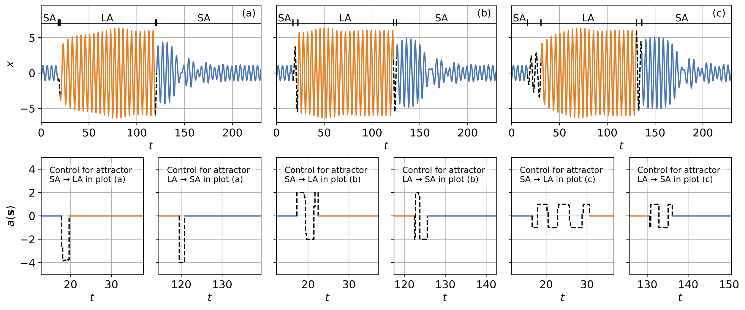
Simulation results in Fig. 3 show the time series of attractor switcing using the control policy learned by the DDPG algorithms. For all three test cases with different action bounds, the Duffing oscillator starts near the SA attractor, then switches from SA to LA, and finally switches backwards from LA to SA.

Several observations:

• Compared with the short time length for control (region of black lines), the attractor switching spends more time waiting for dissipation of the transient process, where the system is automatically approaching the target attractor under no control. Smart strategy learned!!
• Smaller action bound results in a longer time length of control.
• The system quickly approaches near LA when starting from SA, while it takes more time to approach near SA when starting from LA.

Their detailed explanations for these behaviors and the simulation results for CEM can be found in the published paper (see links at the top of this page).