Dynamics of Unforced and Vertically Forced Rocking Elliptical and Semi-Elliptical Disks

• NOTE: This page is a brief introduction of a published work. The detailed information can be found on Journal of Sound and Vibration.

Abstract

• The full equation of motion for both elliptical and semi-elliptical rocking disks is derived from Lagrange’s equation.
• The analysis of equilibrium and stability reveals that the semi-elliptical disk has a super-critical pitchfork bifurcation that enables it to exhibit bistable rocking behavior.
• Both of numerical and experimental investigations unveil nonlinear dynamical behaviors, such as coexisting harmonic and sub-harmonic responses, under vertical excitations.

Background and Motivation

The dynamic behavior of rocking disks is a classical problem that has been studied by scientists, engineers, and mathematicians. This problem was initially studied by Lamb in the early 1900s and followed by several experimental work that validated Lamb’s method for calculating the linear natural frequency of rocking semicircular and parabolic disks. However, these studies focused on linear analysis, and they largely neglected the effects of nonlinearity on the dynamic behavior of the disk.

Another perspective that has not yet been fully investigated is the behavior of rocking disks under vertical excitations. Due to the geometry of an elliptical or semi-elliptical rocking disk, a small vertical excitation can be transferred into magnified rotational movements, which brings potential benefits to the space-efficient energy harvesting. This work shows how nonlinearity significantly influences the dynamics of rocking elliptical and semi-elliptical disks through bifurcations and amplitude-dependent phenomena.

Equations of Motion

As shown in Fig. 1, the disk is rocking on a flat surface which has a prescribed sinusoidal velocity \(\dot{\Gamma}(t) = A \cos {(\Omega t)}\). The surfaces of the disks are defined by \(x^{2}/a^{2} + y^{2}/b^{2} = 1\), where \(a\) and \(b\) are the major and minor radii of the disks, respectively. It’s assumes that the disk has a uniform density and rolls without slip on the base. When deriving the equation of motion, the case of the semi-elliptical disk was used, since the governing equation for the elliptical disk can be obtained from the governing equation for the semi-elliptical disk through two parameter substitutions (will talk it later).

Figure 1. Schematic of a rocking semi-elliptical disk showing both the upright and displaced positions of the object. The disk is vertically excited by the base with a sinusoidal velocity.

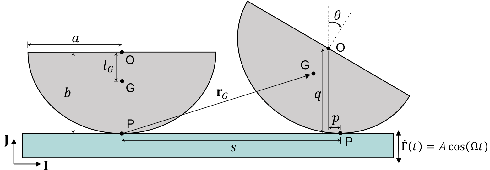
The equation of motion was derived by Lagrange’s equation with \(\theta\) as the generalized coordinate:

\[\ddot \theta + c\dot{\theta} + \frac{K_B}{K_A}\dot \theta ^2 + \frac{l_G \sin \theta + p}{K_A} \left[ {g - A\Omega \sin \left( {\Omega t} \right)} \right] = 0,\]

where

\[\begin{align} K_{A} = & \,\, \kappa^{2} + \left( p + l_G \sin{\theta} \right)^{2} + \left( \frac{a^{2} b^{2}}{q^{3}} -w - l_G \cos{\theta}\right)^{2}, \\ K_{B} = & \,\,\left( \frac{a^{2} b^{2}}{q^{3}} - w - l_G \cos{\theta} \right) \left( 4 p + l_G \sin{\theta} + \frac{3 p w}{q} - \frac{3 a^{2} b^{2} p }{q^{4}} \right)\\ & + \left( p + l_G \sin{\theta} \right) \left( w + l_G \cos{\theta} \right). \end{align}\]

\(c\) is the coefficient of damping which is assumed to be viscous, \(g\) is the gravitational constant, and \(\kappa\) is the disk’s radius of gyration. All other parameters (such as \(a,\,b,\,p,\,q,\,l_G,\,\)etc.) have geometric meanings which can be found in Fig. 1. Due to geometric similarities, this equation of motion describes not only the rocking motion of the semi-elliptical disk, but also that of the elliptical disk by substituting two parameters \(\kappa\) and \(l_G\). The detailed derivation of this equation of motion can be found in the published paper (see links at the top of this page).

Equilibrium and Stability

The system’s equilibrium (the static angles of the rocking disk) varies with the disk’s geometry (the major-minor radii ratio \(a/b\)). For the elliptical disk, the system always has stable equilibria at \(\theta = 0\) (upright position) and \(\theta = \pm \pi\) (flip over), and unstable equilibria at \(\theta = \pm \pi/2\). The only special case is \(a/b=1\) (circular disk), where any angle \(\theta\) could be considered as an equilibrium but is neither stable or unstable.

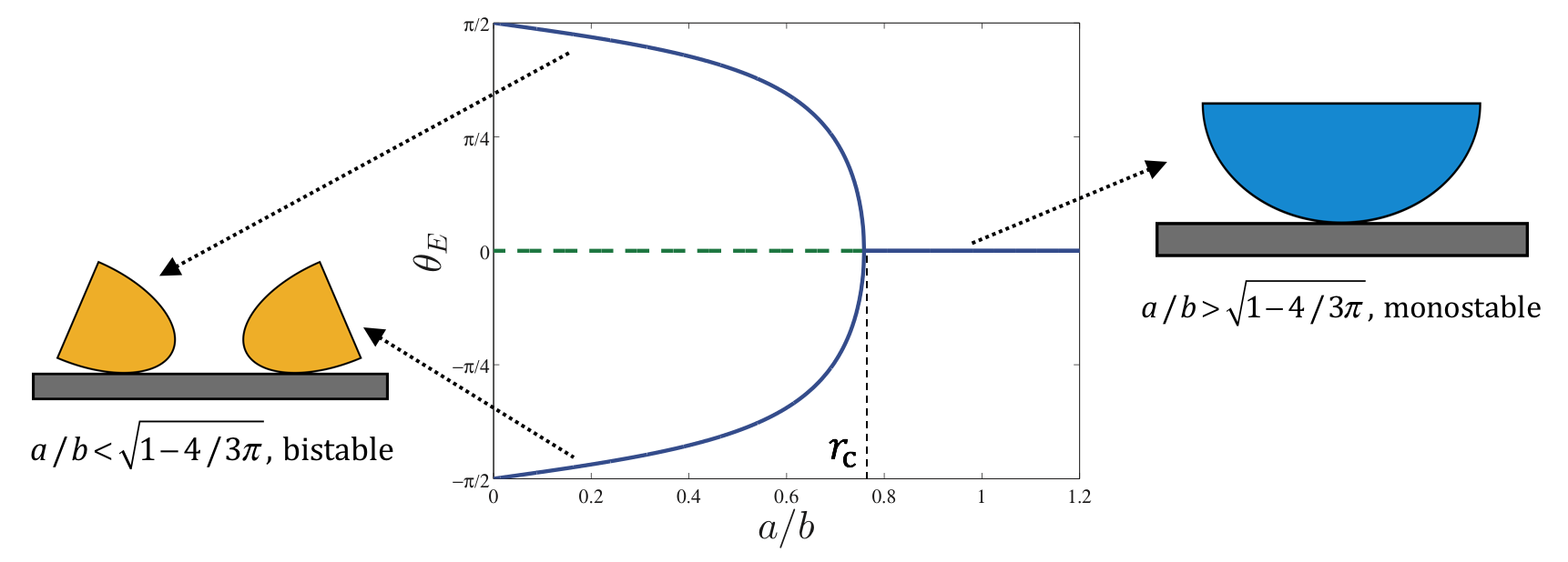
For the semi-elliptical disk, as shown in Fig. 2, there exists a critical value for the \(a\)-to-\(b\) ratio, \(r_\text{c} = \sqrt{1 - 4 / 3 \pi}\). The system has one stable equilibrium position (monostable) at \(\theta = 0\) when \(a/b > r_\text{c}\). A super-critical pitchfork bifurcation occurs at \(a/b = r_\text{c}\), resulting in a reversal of stability for the equilibrium position at \(\theta = 0\) when \(a / b < r_\text{c}\), as well as the creation of two new stable equilibrium (bistable) positions.

Figure 2. Super-critical pitchfork bifurcation diagram showing the stable (solid blue lines) and unstable (dashed green line) equilibria as a function of the dimensionless ratio a/b for the rocking semi-elliptical disk.

More detailed investigations of equilibria and stabilities, including derivation of analytical solutions, phase portraits, basins of attraction and experimental validations, can be found in the published paper (see links at the top of this page).

Dynamic Investigations

The dynamic response of a physical system to varying excitation frequencies is of keen interest in vibration. To provide the frequency response of the rocking disk, the excitation frequency was swept forward and in reverse with numerical simulations. More specifically, the forward and reverse sweep is the linearly increasing and decreasing frequencies with respect to time. Fig. 2 shows the results of frequency sweeping simulations for four different excitation levels.

Figure 2. Forward frequency sweep responses (left column) and reverse frequency sweep responses (right column) for different excitation amplitudes of acceleration: (a, b) 2 m/s², (c, d) 4 m/s², (e, f) 6 m/s², (g, h) 8 m/s². Shaded grey areas represent time series responses and black dots represent stroboscopic samples. The yellow-filled areas denote when the disk flips over or |θ| > π/2. M1-3 are abbreviations for Modes 1-3, whose dynamical behaviors can be found in Fig. 3.

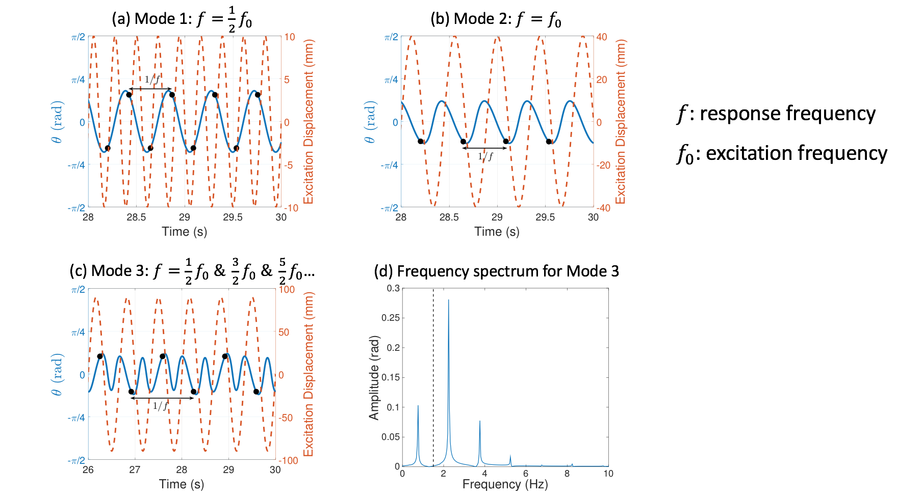
Apart from response frequency and amplitude (grey areas in Fig. 2), stroboscopic samples (black dots in Fig. 2) were also implemented to show the periodicity of the response. Three periodic modes were observed (\(f\) is the disk’s response frequency while \(f_0\) is the excitation frequency):

• Mode 1: \(f=\frac{1}{2}f_0\), a sub-harmonic response where the disk returns to the same position every other excitation period. See Fig. 3(a).
• Mode 2: \(f=f_0\), a harmonic response where the disk rocks back and forth once every excitation period. See Fig. 3(b).
• Mode 3: Multiple frequencies \(f=\frac{1}{2}f_0, \frac{3}{2}f_o, \frac{5}{2}f_o \dots\), where the sub-harmonic response combines with higher frequencies and the stroboscopic points appear identical to Mode 1. See Fig. 3(c, d).

Figure 3. Time series illustrating the three periodic modes. (a)-(c) show the excitation (dashed red line) and the disk's response (solid blue line). Stroboscopic samples (black dots) were overlaid onto the time series. Plot (d) shows the frequency spectrum for Mode 3 with a vertical dashed line at the excitation frequency.

Simulation results above using forward and reverse sweeps demonstrate hysteresis in the rocking disk’s frequency response. More detailed numberical investigations and experimental validations can be found in the published paper (see links at the top of this page).