Nonlinear Dynamics of a Non-Contact Translational-to-Rotational Magnetic Transmission
- NOTE: This page is a brief introduction of a published work. The detailed information can be found on Journal of Sound and Vibration and Nonlinear Structure and Systems.
Abstract
- This work presents an exploratory transmission design to combine three features together: 1) translation-to-rotation, 2) non-contact, and 3) nonlinearity.
- The system’s governing equations were derived under the idealization of a magnetic dipole, and were used to obtain analytical expressions for the system’s equilibria and stabilities.
- Theoretical, numerical and experimental investigations all unveil nonlinear dynamical behaviors, such as coexisting harmonic, sub-harmonic, and chaotic responses, under sinusoidal excitation.
Background and Motivation
The conversion of translational motion into rotational motion, and vice versa, is an important problem area with widespread practical applications and challenges. A primary shortcoming, inherent in systems with mechanical contact and friction, is a reduction in transmission efficiency and the generation of noise. To overcome these shortcomings, various non-contact transmissions were investigated, among which magnetic force is widely used to achieve conversion between rotary and translational motion.
Although various types of magnetic transmission systems have been proposed, considerably less research has embraced their nonlinear behaviors, which are potentially valuable in many applications. For example, in the field of energy harvesting, 1) a non-contact transmission is needed for low friction and high energy efficiency, 2) translation-to-rotation is needed for saving space and connecting to a motor/generator, and 3) nonlinearity is also needed for broad-band frequency responses. This work therefore presents an exploratory transmission design to combine the three features together, and gives a thorough investigation of the system’s static behavior and dynamic responses.
Equations of Motion
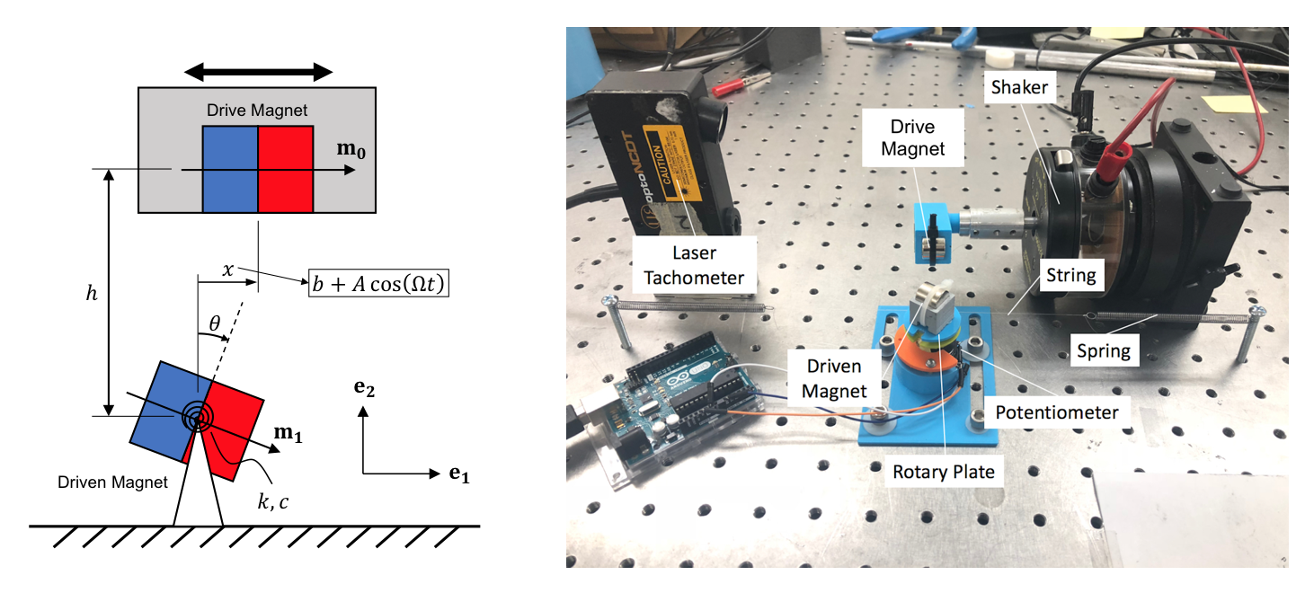
As shown in Fig. 1, the drive magnet is fixed to a vibration source and has a prescribed translational harmonic motion. The driven magnet is pinned and limited to pure rotation about its center of mass. The drive magnet applies a non-contact magnetic force to the driven magnet to achieve translational-to-rotational conversion. In addition to the magnetic force, the driven magnet is also subject to a linear restoring torque from mechanical springs and a damping torque which is assumed to be viscous and proportional to the driven magnet’s angular velocity.
Therefore, the equation of motion can be written as a linear mass-spring-damper system driven by magnetic torque:
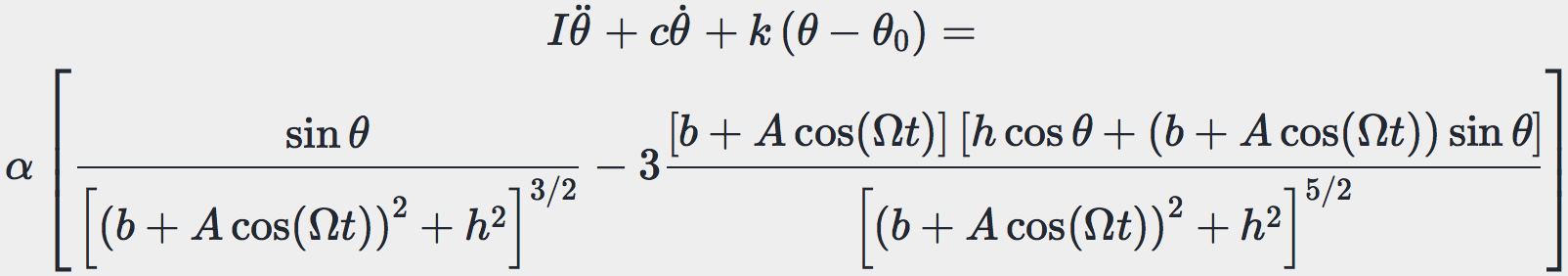
In the LHS, \(I\), \(c\), \(k\) and \(\theta_0\) are the driven magnet’s moment of inertia, torsional spring coefficient, torsional damping coefficient, and offset bias angle of spring respectively. The RHS is the expression of magnetic torque derived by using Dipole model, which is determined by three variables: the angle of the driven magnet \(\theta\), the horizontal distance between two magnets \(x\), which is described by \(b + A\cos(\Omega t)\), and the vertical distance between two magnets \(h\). The factor \(\alpha\) is a constant describing magnetic properties of the drive and driven magnets. The detailed derivation of this equation of motion can be found in the published paper (see links at the top of this page).
Equilibrium and Stability
The system’s equilibrium (i.e., the static angles of the driven magnet) varies with the relative position between the drive and driven magnets. The following two group of animations demonstrate how the equilibrium angle \(\theta\) varies with the vertical distance \(h\) and the horizontal distance \(b\) between the drive and driven magnets.
The offset bias angle \(\theta_0\) in the two cases above was intentionally set a non-zero value (\(\theta_0 = \pi/4\)) to represent inperfection that is inevitable in experiments. More detailed investigations of equilibria and stabilities, including derivation of analytical solutions, bifurcations diagrams for various \(\theta_0\), and experimental validations, can be found in the published paper (see links at the top of this page).
Dynamic Behaviors
The dynamic response of a physical system to varying excitation frequencies is of keen interest in vibration. To provide the frequency response of this transmission system, the excitation frequency was swept forward and in reverse with numerical simulations. More specifically, the forward and reverse sweep is the linearly increasing and decreasing frequencies with respect to time. Fig. 2 shows the results of frequency sweeping simulations for four different excitation amplitudes (\(A =\) 2, 3, 4, 5 mm). In each figure, excitation frequency ranges between \(0.5\omega_\text{n}\) and \(2\omega_\text{n}\), where \(\omega_\text{n}\) is the natural frequency of the transmission system.
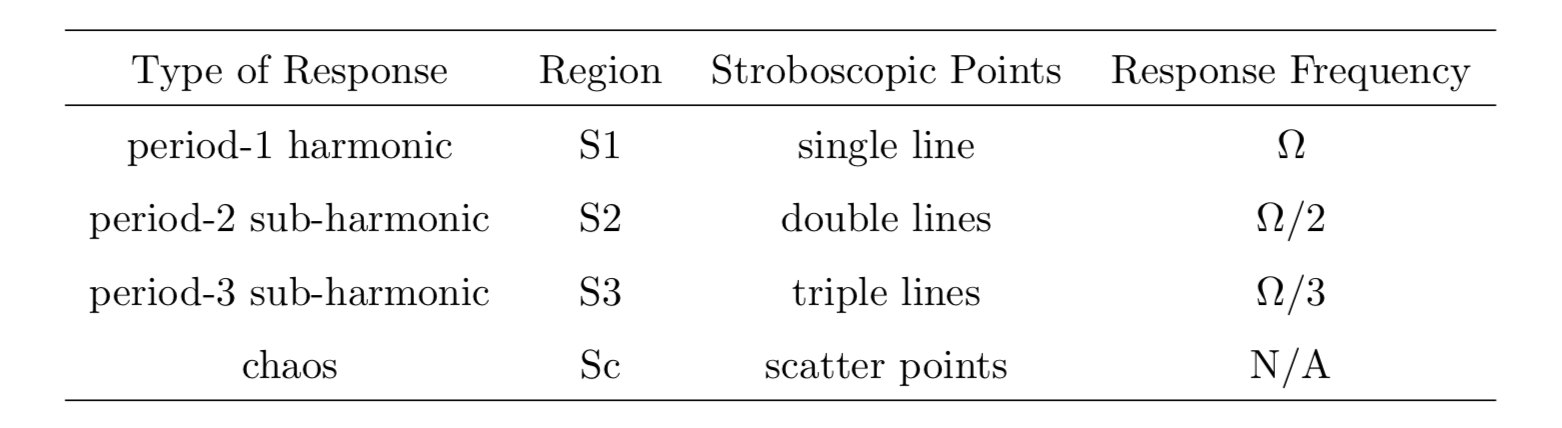
Apart from response frequency and amplitude (grey areas in Fig. 2), stroboscopic samples (black dots in Fig. 2) were also implemented to show the periodicity of the response (see Tab. 1). For example, when the excitation level \(A=4\) mm and the excitation frequency is swept backwards (see Fig. 2(f)), the system exhibits period-1 harmonic, period-2 sub-harmonic, period-3 sub-harmonic and choatic responses.
Simulation results above using forward and reverse frequency sweeps demonstrate multiple periodic responses under the same excitation frequency. However, only two coexisting periodic solutions can be observed in each simulation, i.e. one from the forward sweep and the other one from reverse sweep. This does not consider the chance of finding more coexisting solutions. Therefore, further dynamic investigations were presented in the published paper (see links at the top of this page), including:
- approximate analytical solutions derived using Harmonic Balance,
- experimental validations using the setup shown in Fig. 1.