Model-Free Sampling Method for Basins of Attraction Using Hybird Active Learning

• NOTE: This page is a brief introduction of a research work that will be published soon. The preprint version can be found on arXiv.

Abstract

Understanding the basins of attraction (BoA) is often a paramount consideration for nonlinear systems. This work introduces a model-free sampling method for BoA. The proposed method is based upon hybrid active learning and is designed to find and label the “informative” samples, which efficiently determine the boundary of BoA. It consists of three primary parts:

• Additional sampling on trajectories (AST) to maximize the number of samples obtained from each simulation or experiment.
• An active learning (AL) algorithm to exploit the local boundary of BoA.
• A density-based sampling (DBS) method to explore the global boundary of BoA.

An example of estimating the BoA for a bistable nonlinear system is presented to show the high efficiency of our sampling method.

Background and Motivation

For nonlinear dynamical systems, basins of attraction (BoA) provide a useful mapping from initial conditions to stable equilibria states (attractors). In other words, if the system starts at any state in an attractor’s basin, its trajectory will asymptotically converge to this attractor. An accurate estimation of BoA is of vital importance in analyzing a system’s control stability or predicting its dynamic behavior.

Most existing approaches to determining a high-resolution BoA require prior knowledge of the system’s dynamical model (e.g., differential equation or point mapping for continuous systems, cell mapping for discrete systems, etc.), which allows derivation of approximate analytical solutions or parallel computing on a multi-core computer to find the BoA efficiently. However, there are still several application scenarios where the existing methods work inefficiently or can not be implemented:

• when a continuous map describing the BoA is needed, and
• when the system’s dynamical model is unknown.

For this reason, this work proposes a novel BoA estimation method that can be implemented in such application scenarios. It’s assumed that the BoA boundary is not fractal and the number of attractors is finite. The map describing the BoA can therefore be considered a classifier, identifying to which basin a state belongs. An alternative interpretation of this work is a data-efficient sampling method for training a BoA classifier.

Sampling Method

What’s wrong with the brute-force method?

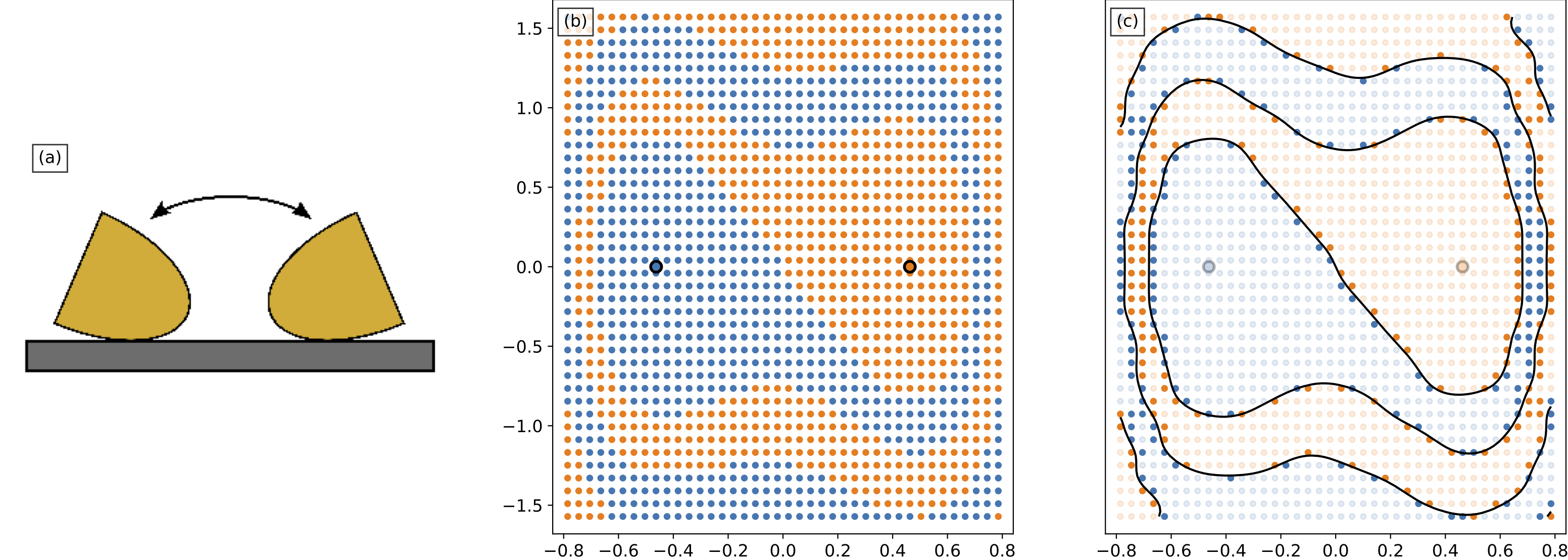
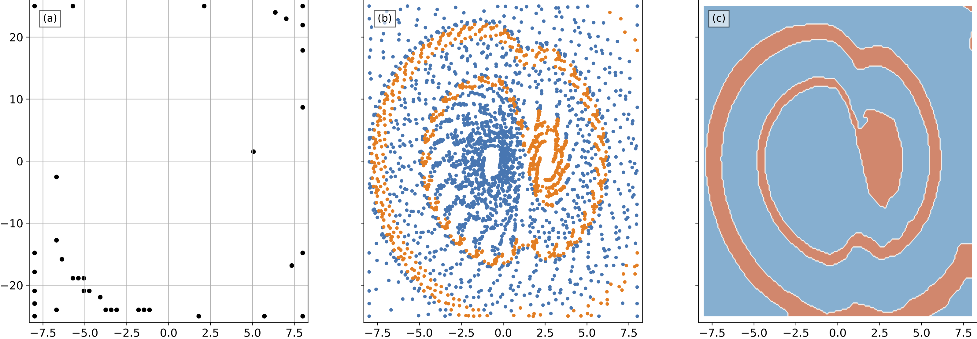
Uniform sampling is a brute-force method to obtain the training data. For the example in Fig. 1, a bistable rocking disk has two equilibria: left-tilt and right-tilt. Its initial angle and angular velocity determine the equilibrium resting angle where it will eventually settle down, thus comprising the system’s BoA. As shown in Fig. 1(b), the uniform sampling method divides the state domain into, e.g., \(40 \times 40\) grids \(= 1600\) samples. Given the fact that BoA is essentially a domain divided into several sub-domains by continuous boundaries, the samples determing the boundaries (i.e. near the boundaries) are more important (or called informative). However, in Fig. 1(c), only the 330 highlighted samples (\(20\%\)) were used to determine the boundary. In other words, uniform sampling wasted \(80\%\) of its workload for uninformative samples.

Figure 1. BoA for a bistable semi-elliptical rocking disk. (a) Two stable equilibria (points circled in black) of the rocking disk: left-tilt and right-tilt. (b) Uniform sampling of 40*40 initial conditions (x-axis for the disks's initial angle, y-axis for its initial angular velocity). The blue and orange points represent the basin of the left-tilt and right-tilt equilibrium respectively. (c) The black line represents the BoA boundary, which is determined by only the highlighted samples (20%). The majority of samples (80%) are far away from the boundary and have no effect on estimating the BoA.

Part 1: Additional Sampling on Trajectories (AST) – Get More Samples for “Free”

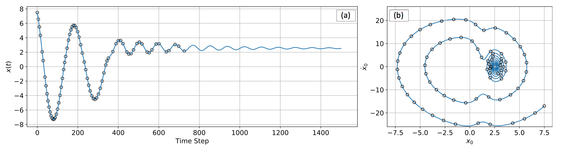
Unlike general classification problems where samples are independent, BoA estimation is able to take advantage of time series trajectories. On a trajectory, every state converges to the same attractor and thus shares the same label. In other words, when the label of an initial condition is determined by one numerical simulation or experiment, the generated time series trajectory can be sub-sampled to obtain additional labeled samples (see Fig. 2).

Figure 2. Additional sampling on trajectories (AST). All the circles are sub-sampled on the same time-series trajectory (blue line), thus sharing the same label (attractor). (a) Additional sampling in time domain. (b) Additional sampling on phase portrait.

Part 2: Active Learning (AL) – Select “Informative” Samples

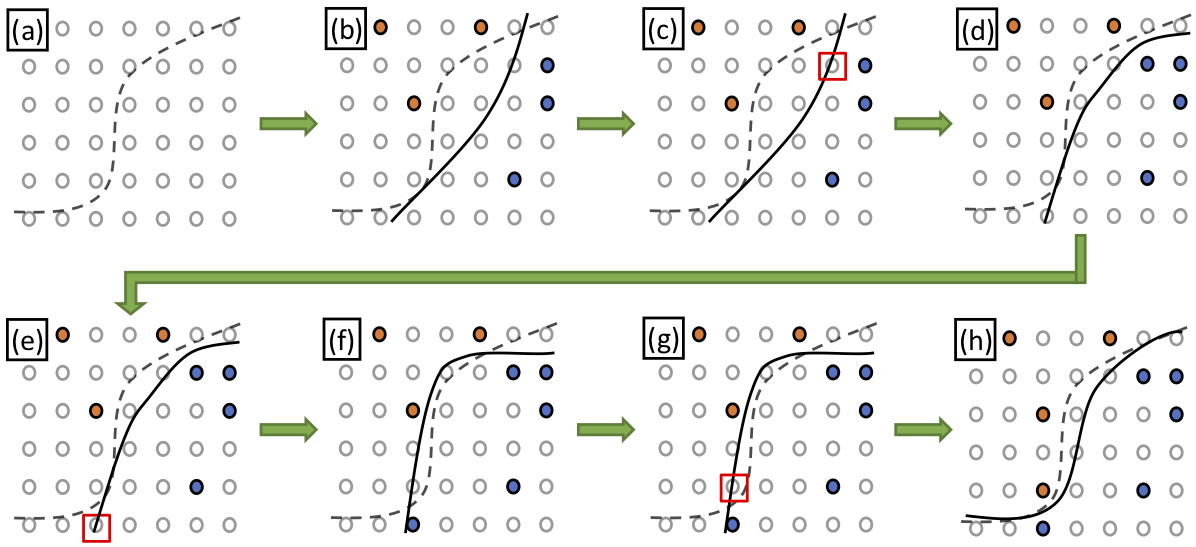
We alrady know that the samples near the boundary are more informative for BoA estimation, but how can we find them without prior knowledge of the boundary? The margin-based active learning (AL) was therefore selected, for it capability of proactively selecting the unlabeled samples most likely to be near a boundary. As shown in Fig. 3, many of labeled samples are located near the real yet unknown classification boundary, which avoids wasted effort on labeling the less informative samples (e.g. the ones at the top-left and bottom-right corners).

Figure 2. Margin-based active learning (AL). The grey dashed line is the real classification boundary while the black lines are the classifiers trained by the labeled samples. (a) Create a pool of unlabeled data. (b) Label a random subset and fit a classifier. (c, e, g) Pick the closest point to the decision boundary. (d, f, h) Label the selected point and fit a new classifier.

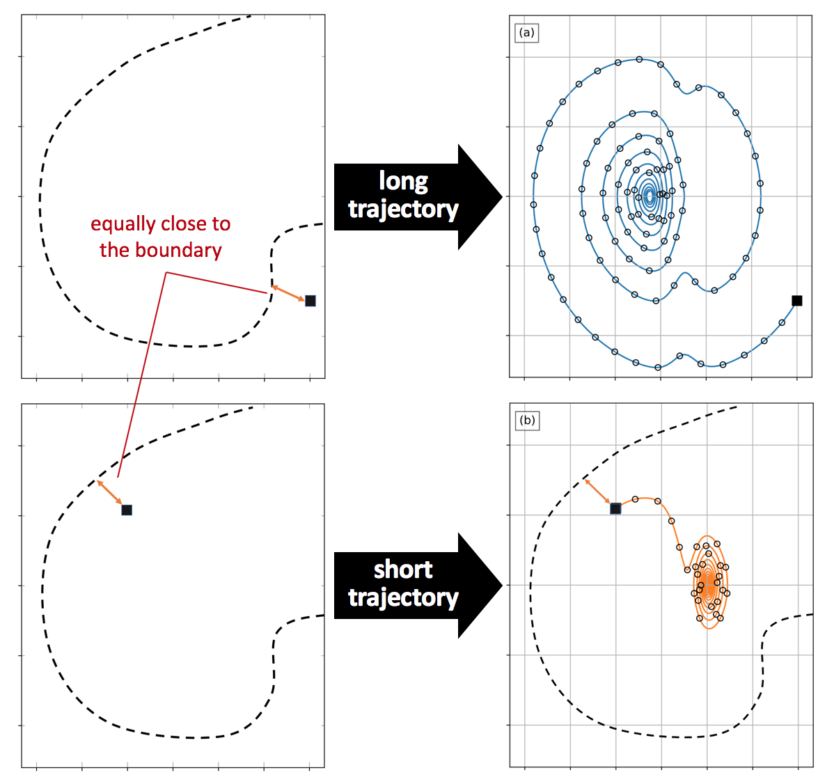
Another question then came out. Is a sample’s “informativeness” only determined by its distance to the boundary? The answer is NO. According to spirit in AST, when multiple samples have a similar distance from the boundary, the length of their trajectories can be used to break the tie (longer trajectories usually provide more additional samples).

As shown in the Fig. 3, when the margin-based AL determines the two unlabeled samples are equally close to the decision boundary, the one in (a) leads to a longer trajectory and more labeled samples, so it has higher priority to be labeled. Since choosing between possible samples requires estimating the lengths prior to generating the trajectories, a predictive model for the trajectory length given a state is needed. A Gaussian process model was selected since it can perform nonlinear regression, has controllable behavior when extrapolating, and needs no prior knowledge of the state distribution.

Figure 3. Unlabeled samples in (a) and (b) are equally close to the boundary, but the sample in (a) leads to more additional samples using AST than (b).

Part 3: Density-Based Sampling (DBS) – Select “Unfamiliar” Samples for Exploration

Similar to the most learning algorithms, our sampling method should also deal with the exploration/exploitation dilemma. A sampling method built upon AL alone tends to exploit only and get stuck in the local BoA boundary. In order to explore the entire state space and estimate the boundary globally, an auxiliary sampling approach based on the density of labeled samples is introduced. This density-based method prioritizes exploring the region in which the fewest samples have been labeled. The detailed implementations of DBS can be found in the original work (see the paper link at the top of this page).

Warp Everything Up

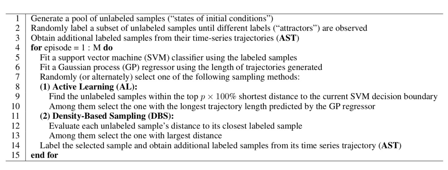
Integrating the three parts above (AST + AL + DBS) leads to a hybrid active learning (HAL) sampling method for estimating BoA (see Tab. 1).

Table 1. Hybrid active learning (HAL) sampling method for estimating basins of attraction (BoA).

Example

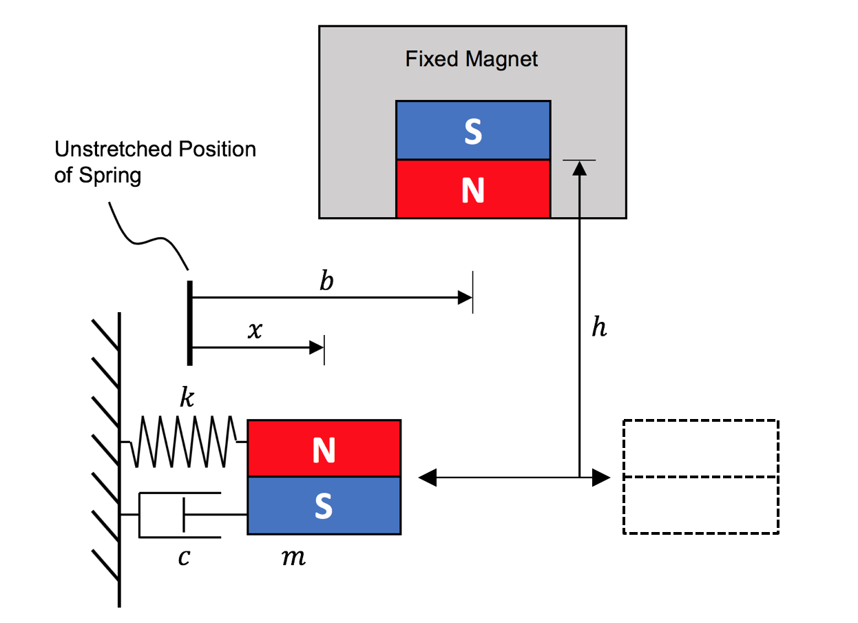
A magnet-induced bistable system in Fig. 4 was used to illustrate the performance of our sampling method. Its governing equation can be written as:

\[m \ddot{x} + c \dot{x} + kx = \frac{\alpha \left( x-b \right) \left[ 12 h^2 - 3 \left( x-b \right) ^2 \right]} {\left[ \left( x-b \right)^2 + h^2 \right]^{7/2}}\]

It’s worth noting that this governing equation has no conflict with the essence of our model-free sampling method. This equation gives simulation results to represent the data collected from experiments, yet was not directly used for the BoA estimation.

Figure 4. Schematic of the magnet-induced bistable system.

The animation below shows our HAL sampling method running on the first 7 episodes. In episode 1-4, HAL looks for the two coexisting attractors (represented by blue and orange respectively). In episode 5-7, the estimated BoA boundary converges to the real one by performing AL and DBS alternately.

After 36 episodes, the total labeled samples are shown in Fig. 5.

Figure 5. (a) The 36 samples selected to be labeled by our hybrid active learning (HAL) sampling method. (b) Additional samples on the time series trajectories generated by using samples in (a) as initial conditions. (c) BoA estimated by a neural network trained with the samples in (b).

Detailed implementations (e.g., including the hyper-parameters in HAL sampling method, the parameters of the magnet-induced bistable system, etc.) and the performance comparison of HAL with other sampling methods can be found in the original work (see the paper link at the top of this page).