Attractor Selection of Nonlinear Energy Harvesting Using Reinforcement Learning

• NOTE: This page is a brief introduction of a research work that will be published soon. The preprint version can be found on arXiv.

Abstract

Recent research efforts demonstrate that the intentional use of nonlinearity enhances the capabilities of energy harvesting systems. One of the primary challenges that arise in nonlinear harvesters is that nonlinearities can often result in multiple attractors with both desirable and undesirable responses that may coexist. In order to ensure the harvester running on the desired attractor (oftentimes the one with maximum power output), this project propose:

• A novel nonlinear energy harvesting system based on a translational-to-rotational magnetic transmission and an electro-magnetic transducer.
• An attractor selection control method based on a reinforcement learning algorithm – deep deterministic policy gradient (DDPG).
• Two controller designs based on a linear actuator and motor voltage respectively.

Background and Motivation

For small and independent devices where replacing battery or integrating in power grid is unrealistic, such as environmental monitoring systems, medical implants and structural health monitoring sensors, vibratory energy harvesters are useful to realize self-powering by converting environmenal mechanical energy to electrical energy. Traditional linear energy harvesters which operate based on linear resonance work well only when excitation frequency is close to the natural frequency. This linear design has a narrow-band frequency response while the energy sources in environment generally have a wide frequency spectrum.

Recent works have suggested the intentional use of nonlinearity might be beneficial to energy harvesting systems, which could exhibit a broader frequency bandwidth than a linear counterpart. However, the introduction of nonlinearity can also cause many additional difficulties. Paramount amongst these challenges, and a common issue in nearly all nonlinear harvesting systems, is the presence of coexisting solutions.

More specifically, for a certain environmental excitation, there exist multiple responses of a harvesting system with various levels of electric power generated. These responses are stable stead-state oscillations, thus also considered “attractors” in nonlinear dynamics. An energy harvester generally prefers running on a high-power attractor for fast energy harvesting, but would also need a low-power attractor for safety reasons or physical restrictions. When one of the attractors is desirable and the other undesirable, it becomes critically important to have a control method to select the desired attractor with minimal energy expenditure.

Energy Harvester Design

Mathematical Model

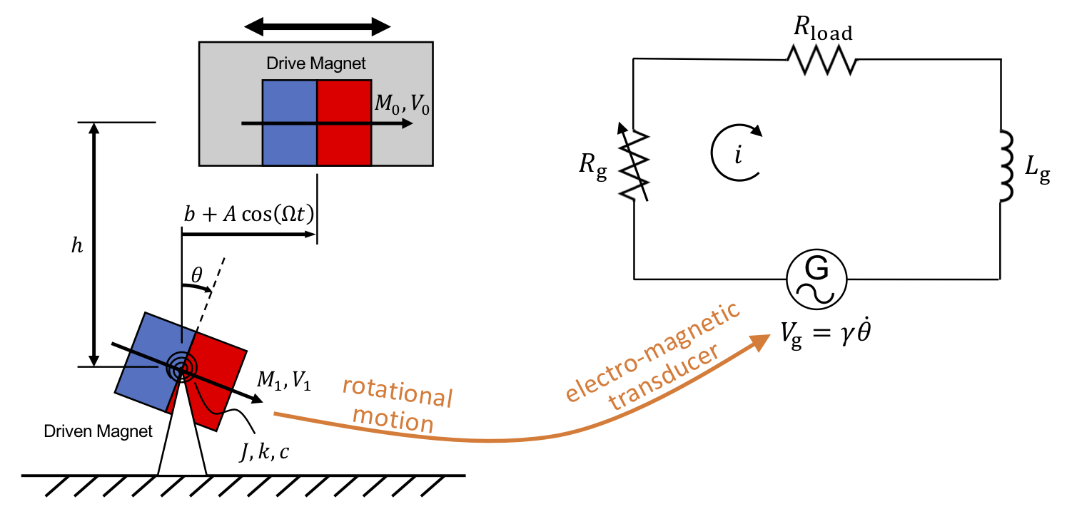
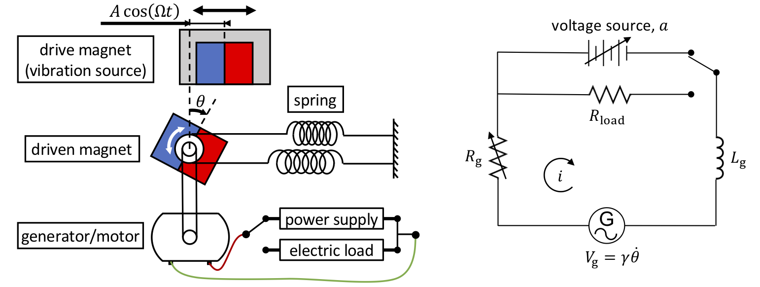
As shown in Fig. 1, the energy harvester is based on a non-contact translational-to-rotational magnetic transmission and an electro-magnetic transducer (such as generator) connecting to a simple resistor load. The governing equation is comprised of 1) the mechanical system’s governing equation where a coupling term \(\gamma i\) was introduced, and 2) an additional equation for the electrical circuit:

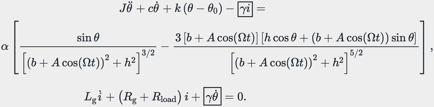
In the left-hand side of the 1st equation, \(J,\, c,\, k\) and \(\theta_0\) are the driven magnet’s moment of inertia, torsional spring coefficient, torsional damping coefficient, and offset bias angle of spring respectively. The right-hand side of the 1st equation is the expression of magnetic torque, which is dependent on the angle of the driven magnet \(\theta\), the vertical distance between two magnets \(h\), and the horizontal distance between two magnets \(b + A\cos(\Omega t)\). A constant \(\alpha\) describes the magnetic properties of magnets. In the 2nd equation, \(R_g\) and \(L_g\) are the resistance and the inductance inside the generator respectively. \(\gamma\) is the electro-mechanical coupling term and \(i\) is the current induced by the rotary motion from the mechanical system. The resistor load \(R_\text{load}\) was used to evaluate the power output.

The detailed derivation of this governing equation and the parameter values used throughout this project can be found in the original work (see the paper link at the top of this page).

Figure 1. Schematic of the energy harvester. The drive magnet is fixed to a vibrational energy source and has a prescribed translational harmonic motion. The driven magnet is pinned and limited to pure rotation about its center of mass. The drive magnet applies a non-contact magnetic force to the driven magnet to achieve translational-to-rotational conversion. This rotation is then conveyed to an electro-magnetic transducer, such as a generator, to produce electric power. In addition to the magnetic force, the driven magnet is also subject to a linear restoring torque from mechanical springs and a viscous damping torque which is assumed to be proportional to the driven magnet's angular velocity.

Coexisting Attractors

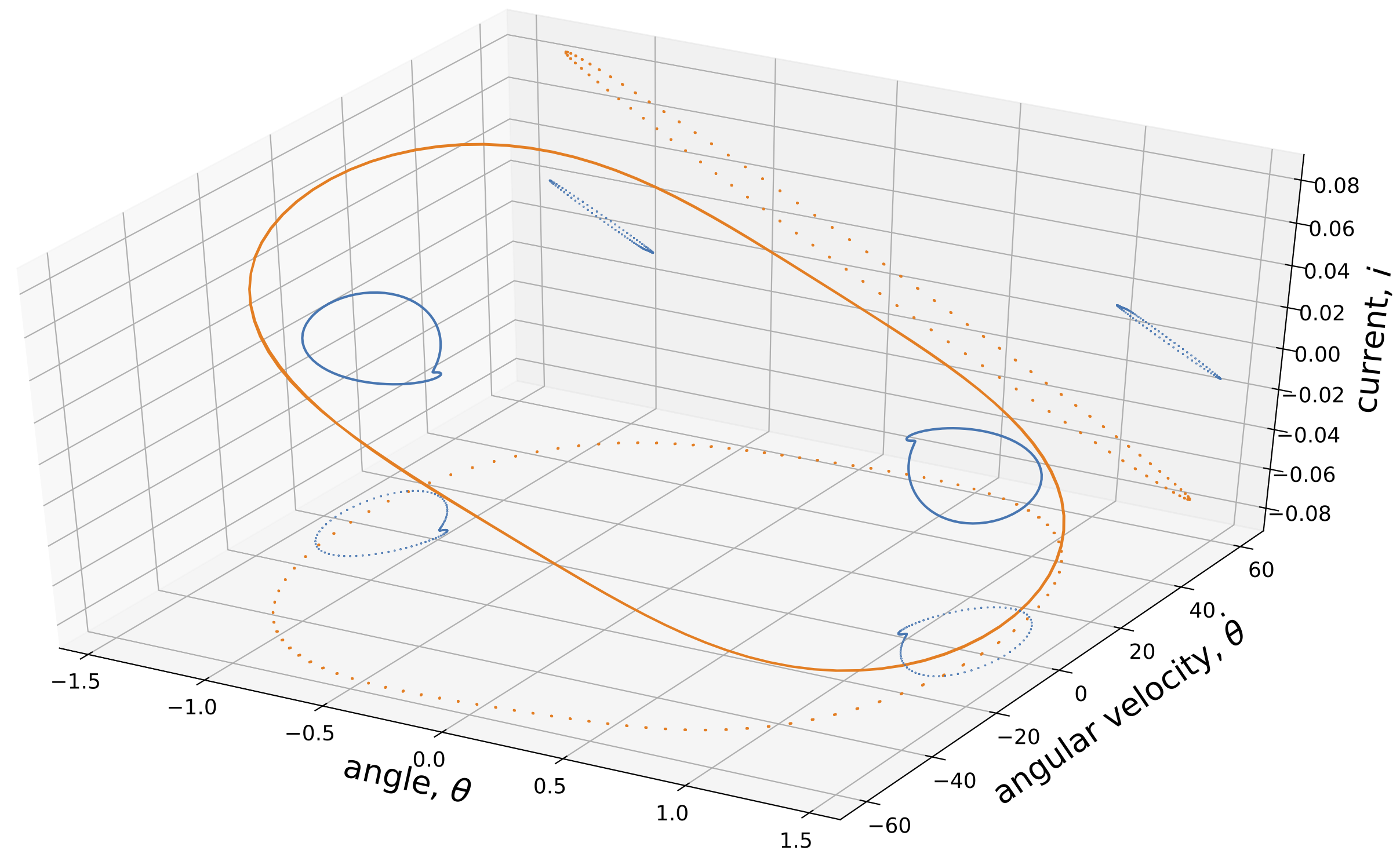
The presence of coexisting attractors is a challenge for nonlinear energy harvesting. Integrating the governing equations with respect to time results in steady-state solutions after initial transient dissipates. These solutions are stable thus they are also considered “attractors” in dynamical systems. The energy harvester has three state variables: the driven magnet’s angle \(\theta\), angular velocity \(\dot{\theta}\) and the induced current \(i\). Thus the phase portraits of steady-state oscillations are closed cycles in 3-dimensional phase domain (see Fig. 2).

Figure 2. Phase portrait of stead-state oscillations of the energy harvester. The orange cycle with a larger oscillation amplitude represents high-power output (HP attractor) while the two symmetric blue cycles with smaller oscillation amplitudes represent low-power output (LP attractor). The dotted lines are the projections of attractors on 2D planes (top view and side view).

Control Option I: Linear Actuator for Moving Spring Position

Controller Design

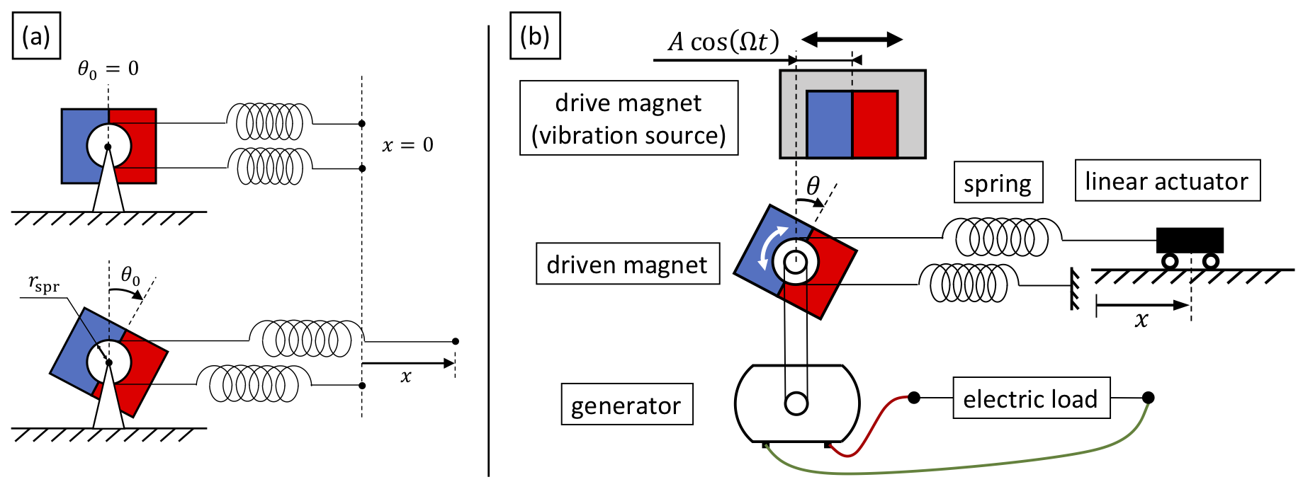
Given that the driven magnet exhibits rotational oscillations while the energy harvester is operating, an reasonable control input is an external torque on the driven magnet. The term \(k\theta_0\) in the governing equation can be considered an external torque that is controllable. This term forms a torque determined by the offset bias angle \(\theta_0\), which is the static equilibrium angle when the system is only forced by springs (see Fig. 3(a)). The offset bias angle \(\theta_0\) can be altered by moving springs, and has a linear relationship with the distance between ends of springs \(x = 2 r_\text{spr} \theta_0\).

In order to manipulate the distance \(x\), as shown in Fig. 3(b), the end of one spring is fixed and that of the other spring is attached to a linear actuator. Instead of directly controlling the actuator’s position \(x\), its velocity \(\dot{x}\) was chosen to be the control input for a more practical control scenario. The system’s governing equation becomes:

\[\begin{equation} \begin{split} I \ddot{\theta} + c \dot{\theta} + k \theta - \gamma i &= \tau_\text{mgt} + \frac{k}{2 r_\text{spr}} x, \\ L_\text{g} \dot{i} + \left( R_\text{g} + R_\text{load} \right) i + \gamma \dot{\theta} &= 0, \\ \dot{x} &= a, \end{split} \end{equation}\]

where \(a\) is the control input – the actuator’s velocity, and \(\tau_\text{mgt}\) is the magnetic torque, i.e., the right hand side of previous governing equation.

Figure 3. Schematic of control option I, where an external torque on the driven magnet is provided by moving spring position with a linear actuator. (a) shows the linear relationship between x and θ₀. In (b), the vibration of the energy source is first transmitted the rotation of the driven magnet, then conveyed to an electro-magnetic transducer (generator) to produce electric power.

Result

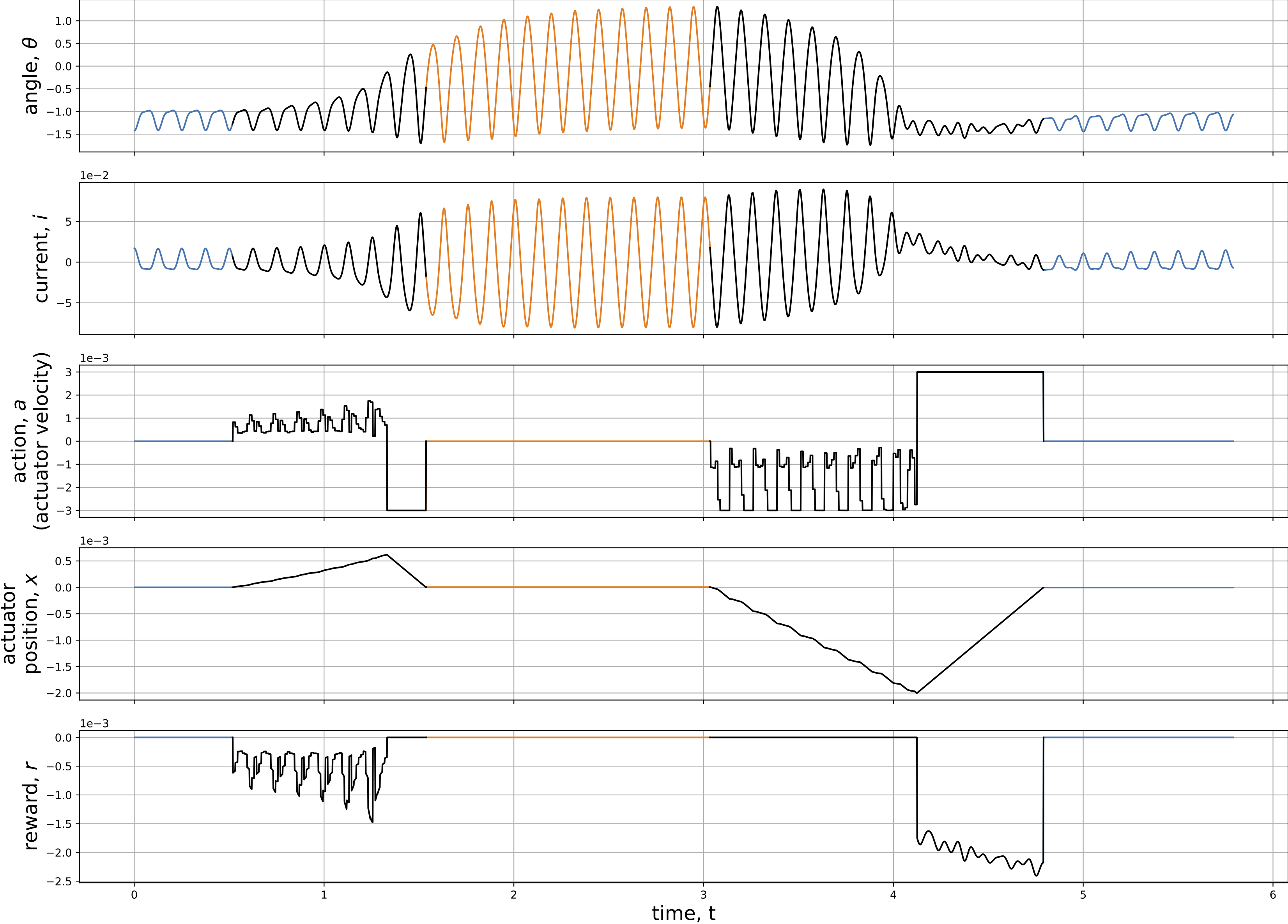
The following animation shows how the energy harvester is controlled by a linear actuator to switch from the LP (low-power) attractor to HP (high-power) attractor. The control policy was learned by using a reinforcement learning algorithm – DDPG (deep deterministic policy gradient). The three plots in the right column are the time series of the driven magnet’s angle \(\theta\), the induced current \(i\) and the actuator displacement \(x\) respectively.

In order to demonstrate the success of attractor switching in both direction: LP-to-HP and HP-to-LP, Fig. 4 includes five stages:

• controller OFF, operating on the LP attractor (blue lines).
• controller ON, switching from LP to HP (black lines).
• controller OFF, waiting for the dissipation of transient process, then operating on the HP attractor (orange lines).
• controller ON, switching from HP to LP (black lines).
• controller OFF, waiting for the dissipation of transient process, then operating on the LP attractor (blue lines).

There are five plots of time series in Fig. 4. The 1st and 2nd plots are the responses of the driven magnet angle and the induced current, which directly tell the attractor from their oscillation amplitudes (large amplitude for HP attractor and small amplitude for LP attractor). The 3rd and 4th plots are the controller’s (linear actuator’s) velocity and displacement respectively, where the velocity is also the control input. The last plot of reward could be interpreted as “action cost”. The area above the curve is the energy consumed for attractor switching.

Figure 4. Time series of the attractor switching using the control option I (spring control) + DDPG. The energy harvester was first switched from LP to HP attractor and then switched back from HP to LP attractor. The blue, orange and black lines represent the system running on the LP attractor, running on the HP attractor, being under control, respectively.

More detailed investigations were presented in the published paper (see links at the top of this page), including:

• The detailed implementation of reinforcement learning to the attractor selection problem.
• Observations and analyses from the time series in Fig. 4.
• A quasi-bang-bang control method based on simplifying and imitating the DDPG-based control policy.

Control Option II: External Voltage on the Motor

Controller Design

The energy harvester’s attractors are steady-state oscillations determined by three state variables: the driven magnet’s angle \(\theta\), angular velocity \(\dot\theta\) and induced current \(i\). Apart from exerting an external torque to control the angle and velocity using an actuator (controll option I), the induced current could also be controlled by introducing an external power supply in the electro-magnetic circuit. As shown in Fig. 5, while the energy harvester is operating on an attractor, the generator is driven by the rotating magnet and powering an electric load. When the energy harvester is going to switch to another attractor, the generator is detached from the electric load and connected to a power supply, thus becoming a “motor” to reversely drive the rotating magnet. The circuit will be switched back to connect the electric load once the target attractor is reached.

Figure 5. Schematic of control option II (voltage control).

The system’s governing equation becomes:

\[\begin{split} I \ddot{\theta} + c \dot{\theta} + k \theta - \gamma i &= \tau_\text{mgt}, \\ L_\text{g} \dot{i} + R_\text{g} i + \gamma \dot{\theta} &= \begin{cases} a, & \text{if controller is ON}\\ - R_\text{load} i, & \text{if controller is OFF} \end{cases} \end{split}\]

where \(a\) is the control input of voltage and the controller is switched ON & OFF by using a relay as shown in Fig. 5.

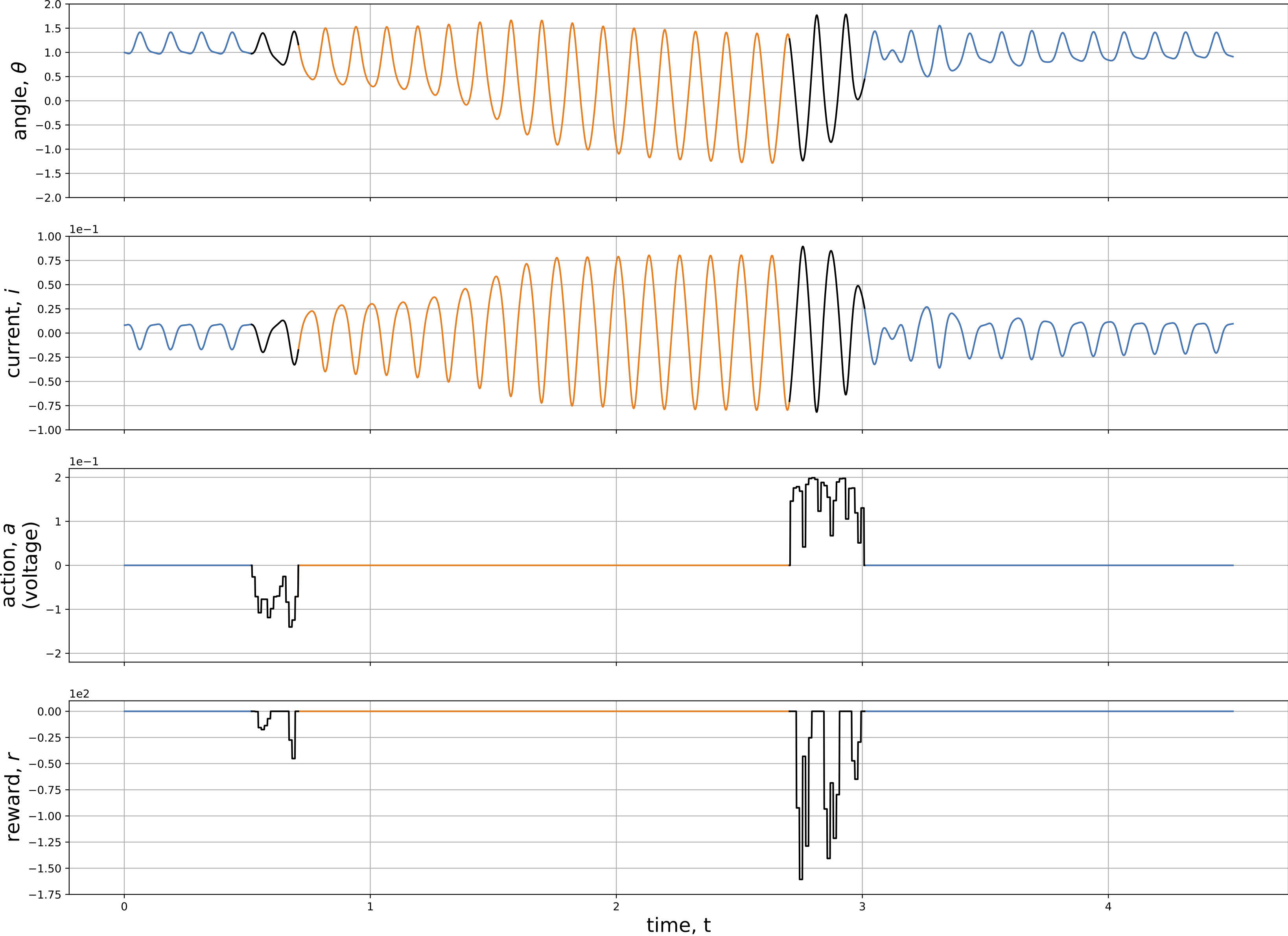
Result

Like what was done for the controller I (spring control), the control policies for attractor switching in both directions (LP-to-HP and HP-to-LP) were learned by using the reinforcement learning algorithm – DDPG. Fig. 6 shows the time series of the switching process. The 1st and 2nd plots are the time series response of the energy harvester: the driven magnet angle \(\theta\) and the induced current \(i\) respectively. The 3rd plot is for the control input, i.e., the voltage on the motor. Last, in the reward plot, the areas above the curve represent the energy consumed for attractor switching.

Figure 6. Time series of the attractor switching using the control option II (motor voltage). The energy harvester governed was first switched from LP to HP attractor and then switched back from HP to LP attractor. The blue, orange and black lines represent the system running on the LP attractor, running on the HP attractor, being under control, respectively.

More detailed investigations were presented in the published paper (see links at the top of this page), including:

• How to define the reward function in reinforcement learning to minimize the energy consumption for attractor switching.
• Performance of the control option II (voltage control) with various action bounds, i.e., the maximum control voltage allowed.
• Comparison of the control option I (spring control) and control option II (voltage control).